What Does Geom_col() Do? How Is It Different to Geom_bar()
There are two types of bar charts: geom_bar() and geom_col(). geom_bar() makes the top of the bar proportional to the number of cases in each grouping (or if the weight aesthetic is supplied, the sum of the weights). If you want the heights of the bars to correspond values in the information, utilise geom_col() instead. geom_bar() uses stat_count() by default: information technology counts the number of cases at each ten position. geom_col() uses stat_identity(): it leaves the data as is.
Usage
geom_bar ( mapping = Nil, data = Null, stat = "count", position = "stack", ..., width = NULL, na.rm = Simulated, orientation = NA, show.legend = NA, inherit.aes = TRUE ) geom_col ( mapping = Naught, data = NULL, position = "stack", ..., width = NULL, na.rm = Simulated, show.legend = NA, inherit.aes = True ) stat_count ( mapping = Zippo, information = Goose egg, geom = "bar", position = "stack", ..., width = NULL, na.rm = FALSE, orientation = NA, show.legend = NA, inherit.aes = Truthful ) Arguments
- mapping
-
Gear up of aesthetic mappings created past
aes()oraes_(). If specified andinherit.aes = TRUE(the default), it is combined with the default mapping at the meridian level of the plot. You must supplymappingif at that place is no plot mapping. - data
-
The information to exist displayed in this layer. There are three options:
If
NULL, the default, the information is inherited from the plot data as specified in the phone call toggplot().A
information.frame, or other object, will override the plot information. All objects will be fortified to produce a data frame. Seefortify()for which variables will be created.A
partwill be chosen with a unmarried argument, the plot data. The return value must be adata.frame, and will be used as the layer data. Afunctioncan be created from aformula(eastward.g.~ head(.10, 10)). - position
-
Position adjustment, either as a cord, or the result of a phone call to a position aligning function.
- ...
-
Other arguments passed on to
layer(). These are oft aesthetics, used to set an aesthetic to a fixed value, likecolour = "red"orsize = iii. They may also be parameters to the paired geom/stat. - width
-
Bar width. By default, set to 90% of the resolution of the data.
- na.rm
-
If
False, the default, missing values are removed with a warning. IfTRUE, missing values are silently removed. - orientation
-
The orientation of the layer. The default (
NA) automatically determines the orientation from the aesthetic mapping. In the rare event that this fails it tin can be given explicitly by settingorientationto either"x"or"y". See the Orientation section for more detail. - show.fable
-
logical. Should this layer exist included in the legends?
NA, the default, includes if any aesthetics are mapped.Falsenever includes, andTRUEever includes. It can also be a named logical vector to finely select the aesthetics to brandish. - inherit.aes
-
If
Simulated, overrides the default aesthetics, rather than combining with them. This is nearly useful for helper functions that define both information and aesthetics and shouldn't inherit behaviour from the default plot specification, eastward.grand.borders(). - geom, stat
-
Override the default connection betwixt
geom_bar()andstat_count().
Details
A bar chart uses height to represent a value, and and then the base of operations of the bar must e'er be shown to produce a valid visual comparison. Go along with caution when using transformed scales with a bar chart. Information technology'south of import to always use a meaningful reference point for the base of the bar. For instance, for log transformations the reference point is 1. In fact, when using a log scale, geom_bar() automatically places the base of operations of the bar at 1. Furthermore, never use stacked bars with a transformed scale, because scaling happens earlier stacking. Equally a consequence, the height of bars volition exist incorrect when stacking occurs with a transformed scale.
By default, multiple bars occupying the same x position will be stacked atop one another by position_stack(). If you lot want them to be dodged side-to-side, apply position_dodge() or position_dodge2(). Finally, position_fill() shows relative proportions at each x past stacking the bars and then standardising each bar to take the same height.
Orientation
This geom treats each axis differently and, thus, can thus have two orientations. Often the orientation is easy to deduce from a combination of the given mappings and the types of positional scales in utilize. Thus, ggplot2 will by default try to guess which orientation the layer should accept. Under rare circumstances, the orientation is ambiguous and guessing may neglect. In that case the orientation tin can be specified directly using the orientation parameter, which can be either "ten" or "y". The value gives the axis that the geom should run along, "x" being the default orientation you would await for the geom.
Aesthetics
geom_bar() understands the following aesthetics (required aesthetics are in bold):
-
x -
y -
alpha -
color -
fill -
group -
linetype -
size
Learn more about setting these aesthetics in vignette("ggplot2-specs").
geom_col() understands the following aesthetics (required aesthetics are in bold):
-
x -
y -
alpha -
colour -
make full -
group -
linetype -
size
Learn more than nigh setting these aesthetics in vignette("ggplot2-specs").
stat_count() understands the post-obit aesthetics (required aesthetics are in bold):
-
10ory -
group -
weight
Learn more nearly setting these aesthetics in vignette("ggplot2-specs").
Computed variables
- count
-
number of points in bin
- prop
-
groupwise proportion
Run across as well
geom_histogram() for continuous information, position_dodge() and position_dodge2() for creating side-by-side bar charts.
stat_bin(), which bins information in ranges and counts the cases in each range. Information technology differs from stat_count(), which counts the number of cases at each x position (without binning into ranges). stat_bin() requires continuous x data, whereas stat_count() can be used for both discrete and continuous 10 information.
Examples
# geom_bar is designed to make it easy to create bar charts that show # counts (or sums of weights) 1000 <- ggplot ( mpg, aes ( grade ) ) # Number of cars in each class: yard + geom_bar ( ) 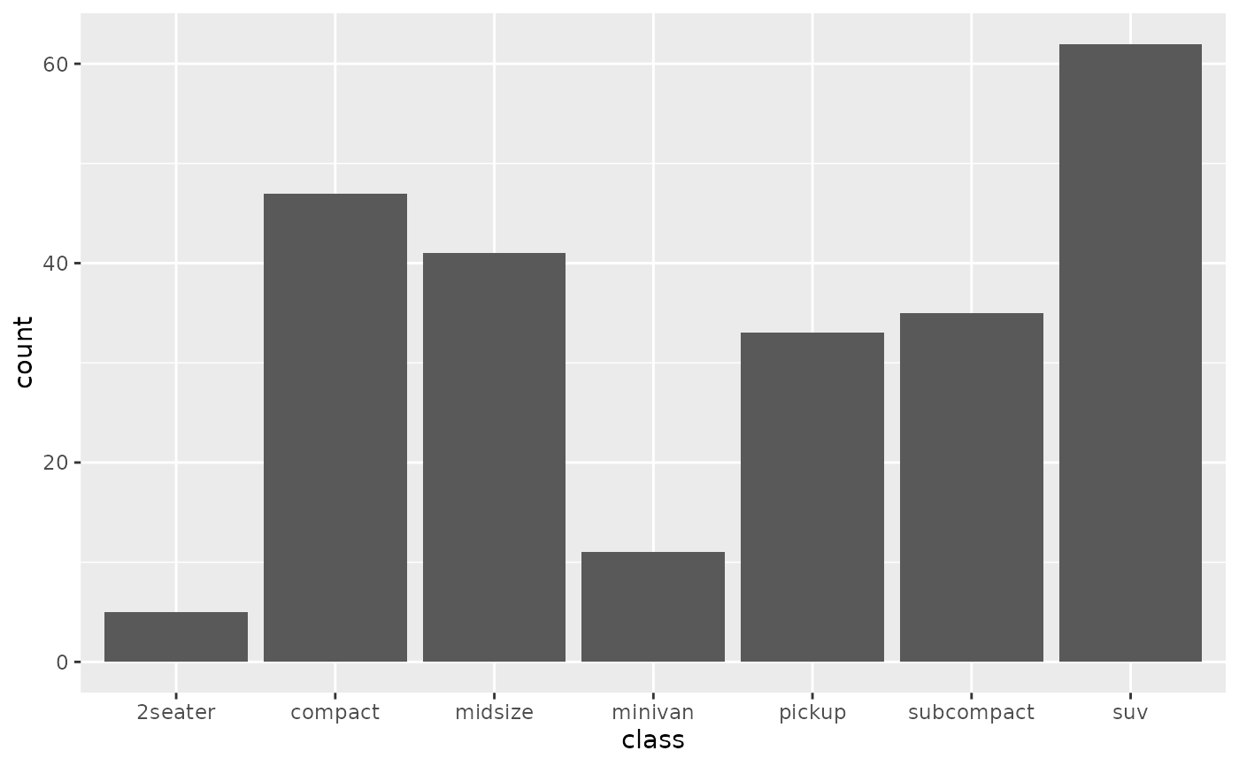 # Full engine displacement of each form g + geom_bar ( aes (weight = displ ) )
 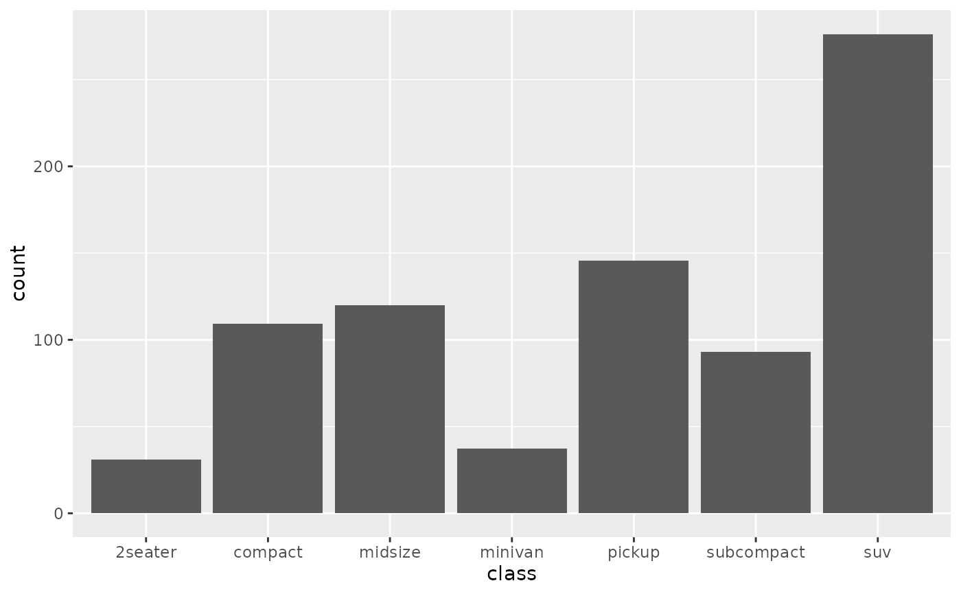 # Map form to y instead to flip the orientation ggplot ( mpg ) + geom_bar ( aes (y = class ) )
 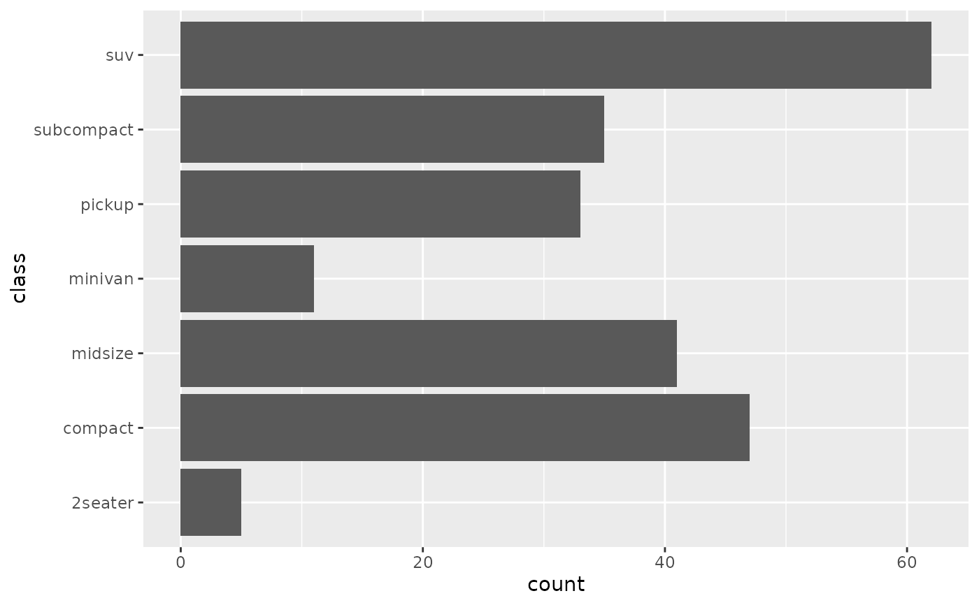 # Bar charts are automatically stacked when multiple confined are placed # at the same location. The order of the fill up is designed to match # the legend g + geom_bar ( aes (fill = drv ) )
 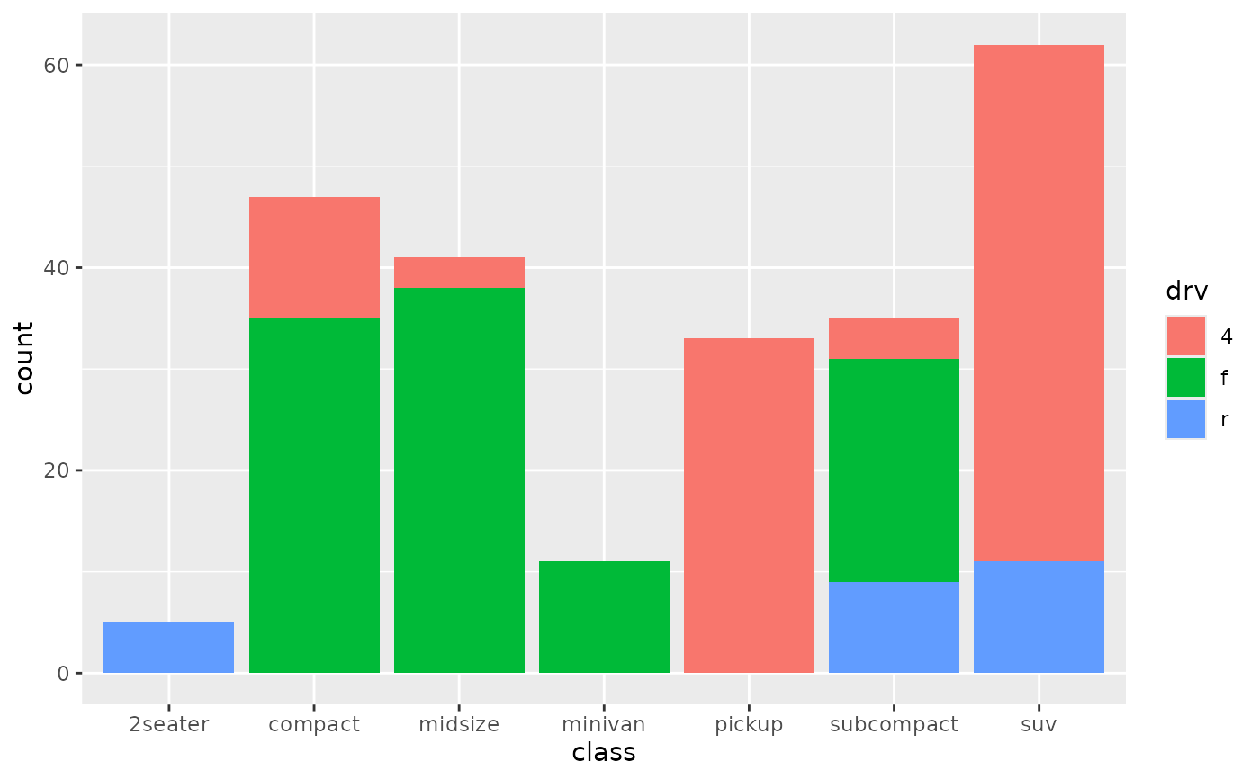 # If you need to flip the order (because you've flipped the orientation) # call position_stack() explicitly: ggplot ( mpg, aes (y = class ) ) + geom_bar ( aes (fill = drv ), position = position_stack (contrary = Truthful ) ) + theme (legend.position = "top" )
 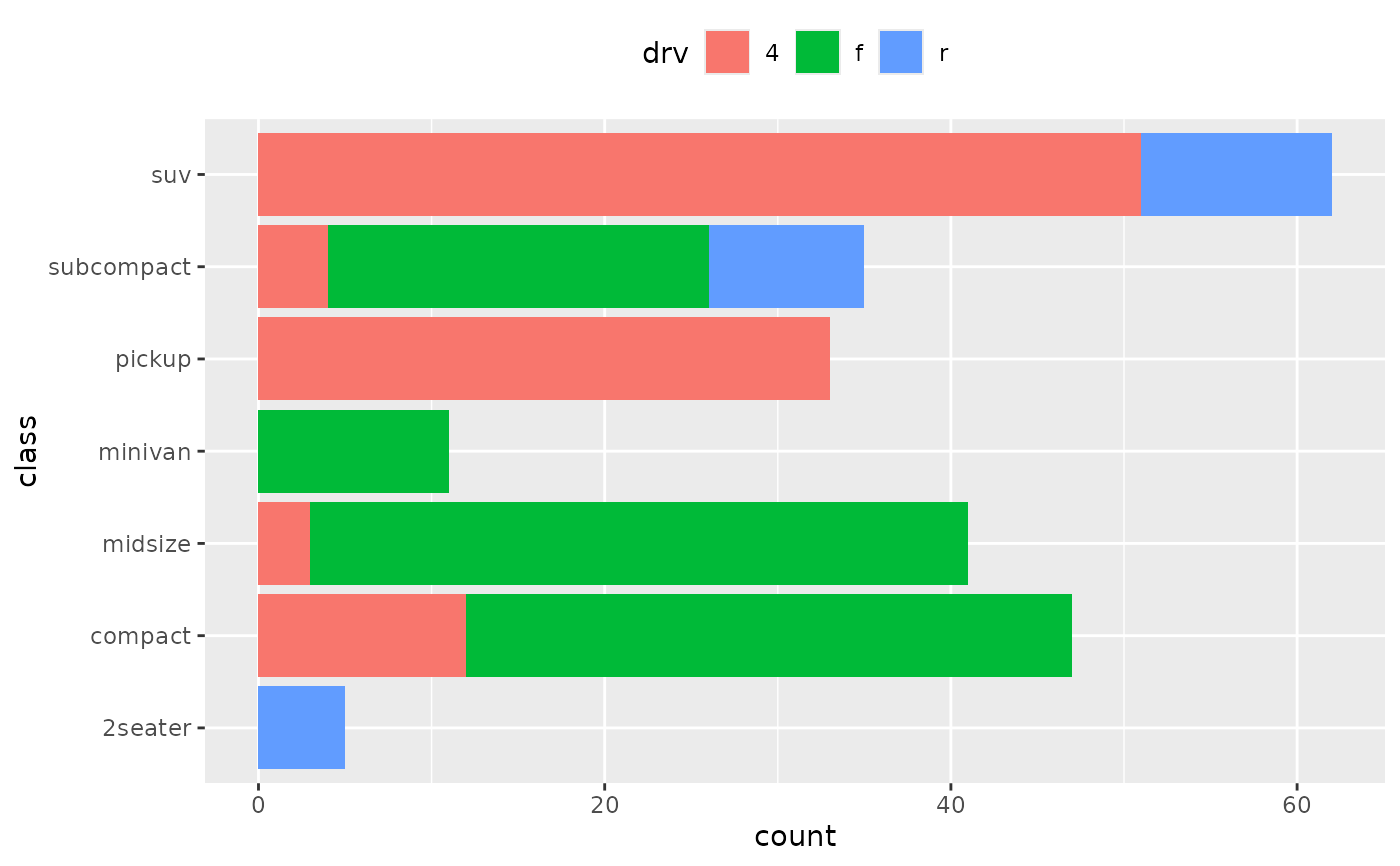 # To prove (eastward.g.) means, you demand geom_col() df <- data.frame (trt = c ( "a", "b", "c" ), event = c ( 2.iii, 1.9, 3.2 ) ) ggplot ( df, aes ( trt, outcome ) ) + geom_col ( )
 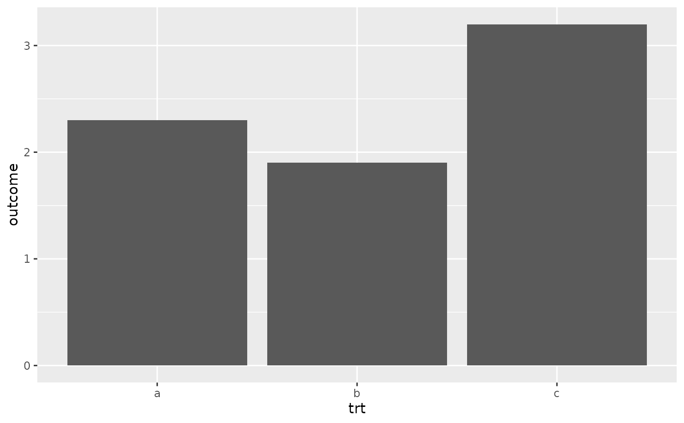 # But geom_point() displays exactly the same information and doesn't # require the y-axis to affect zero. ggplot ( df, aes ( trt, outcome ) ) + geom_point ( )
 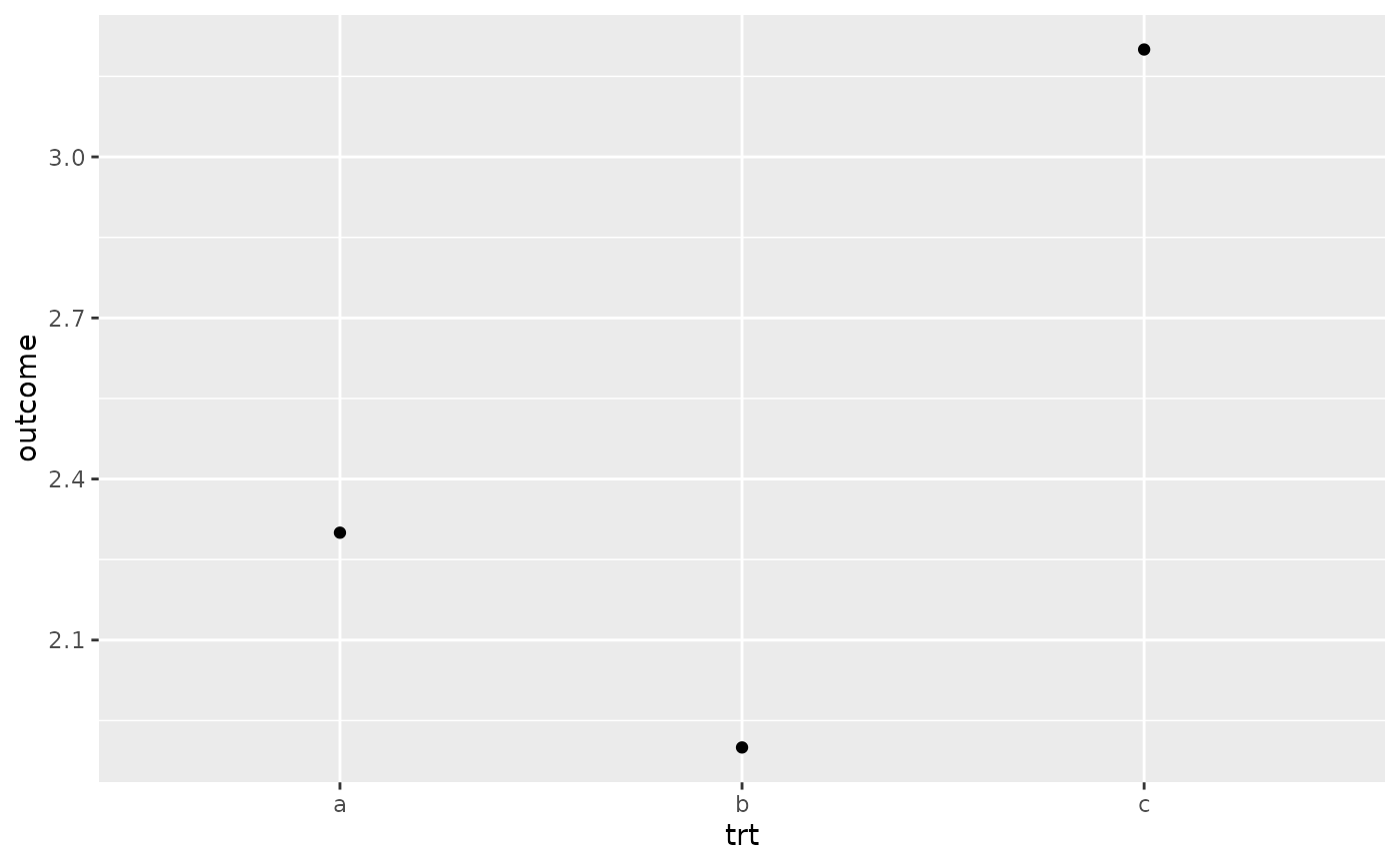 # You can besides use geom_bar() with continuous data, in which case # information technology volition show counts at unique locations df <- information.frame (ten = rep ( c ( 2.9, 3.1, iv.5 ), c ( 5, 10, 4 ) ) ) ggplot ( df, aes ( x ) ) + geom_bar ( )
 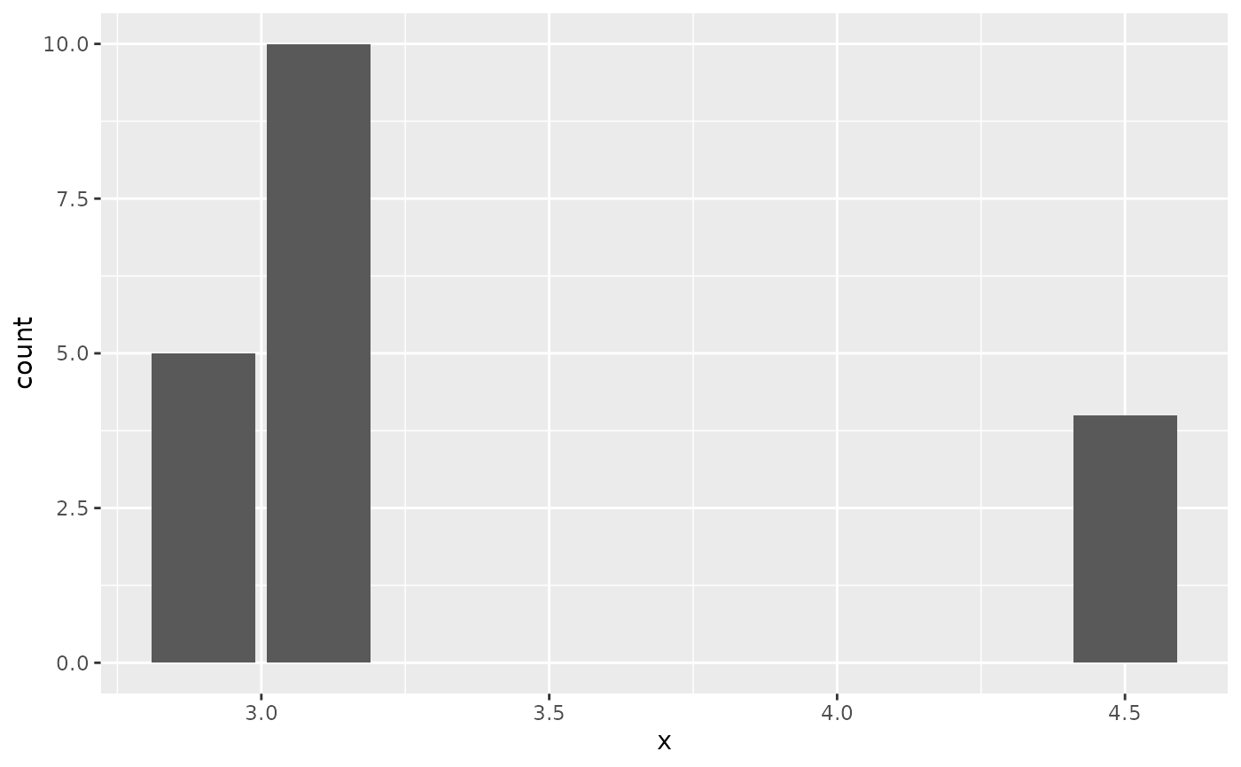 # cf. a histogram of the aforementioned data ggplot ( df, aes ( 10 ) ) + geom_histogram (binwidth = 0.5 )
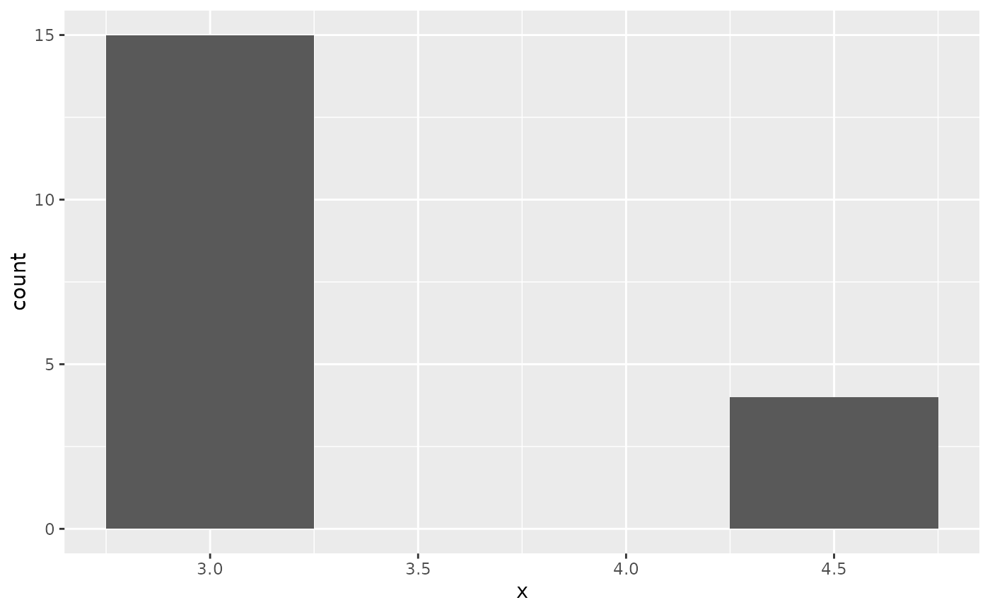
Source: https://ggplot2.tidyverse.org/reference/geom_bar.html
 Do? How Is It Different to Geom_bar())
Post a Comment for "What Does Geom_col() Do? How Is It Different to Geom_bar()"